三、pandas-Series-案例 （1）学生成绩统计创建一个包含10名学生成绩的Series，成绩范围在50 - 100之间。计算平均分、最高分、最低分，并找出高于平均分的学生人数。import numpy as np import pandas as pd # 生成随机成绩 np.random.seed(1) scores = pd.Series(np.random.randint(50, 101, 10), index=['学生' + str(i) for i in range(1, 11)]) print(scores) 学生1 87 学生2 93 学生3 62 学生4 58 学生5 59 学生6 61 学生7 55 学生8 65 学生9 50 学生10 66 dtype: int32mean_score = scores.mean() print("平均分：", mean_score) print("最高分：", scores.max()) print("最低分：", scores.min()) print("成绩高于平均分的学生人数：", scores[scores > mean_score].count()) 平均分： 65.6 最高分： 93 最低分： 50 成绩高于平均分的学生人数： 3（2）温度数据分析给定某城市一周中每天的最高温度Series，计算温度超过30°的天数，平均温度，温度由高到低排序，并找出温度变化最大的两天import numpy as np import pandas as pd # 温度 temperature = pd.Series([28, 26, 33, 31, 32, 30, 27], index=['周一', '周二', '周三', '周四', '周五', '周六', '周日', ]) print(temperature) 周一 28 周二 26 周三 33 周四 31 周五 32 周六 30 周日 27 dtype: int64print("温度超过30°的天数：", temperature[temperature > 30].count()) print("平均温度：", round(temperature.mean(), 1)) # ascending=False 降序 temperature_sort = temperature.sort_values(ascending=False) print(temperature_sort) # 计算相邻两天的温度差值 temperature_diff = temperature.diff().abs() temperature_diff_sort = temperature_diff.sort_values(ascending=False) print("温度变化最大的两天：", temperature_diff_sort.index[:2].tolist()) 温度超过30°的天数： 3 平均温度： 29.6 周三 33 周五 32 周四 31 周六 30 周一 28 周日 27 周二 26 dtype: int64 温度变化最大的两天： ['周三', '周日']（3）股票价格分析给定某股票连续10个交易日的收盘价Series，计算每日收益率（当日收盘价/前日收盘价 - 1），找出收益率最高和最低的日期，计算波动率（收益率标准差）import numpy as np import pandas as pd prices = pd.Series([105.2, 103.1, 104.6, 102.9, 101.9, 106, 108.2, 105.1, 104.6, 102.9], index=pd.date_range('2025-10-01', periods=10)) print(prices) 2025-10-01 105.2 2025-10-02 103.1 2025-10-03 104.6 2025-10-04 102.9 2025-10-05 101.9 2025-10-06 106.0 2025-10-07 108.2 2025-10-08 105.1 2025-10-09 104.6 2025-10-10 102.9 Freq: D, dtype: float64print("收益率：") pct_change = prices.pct_change() print(pct_change) print("收益率最高的日期：", pct_change.idxmax()) print("收益率最低的日期：", pct_change.idxmin()) print("波动率：", pct_change.std()) 收益率： 2025-10-01 NaN 2025-10-02 -0.019962 2025-10-03 0.014549 2025-10-04 -0.016252 2025-10-05 -0.009718 2025-10-06 0.040236 2025-10-07 0.020755 2025-10-08 -0.028651 2025-10-09 -0.004757 2025-10-10 -0.016252 Freq: D, dtype: float64 收益率最高的日期： 2025-10-06 00:00:00 收益率最低的日期： 2025-10-08 00:00:00 波动率： 0.022586890620196715（4）销售数据分析某产品过去12个月的销售量Series，计算季度平均销量，销量最高的月份，月环比增长率，连续增长超过两个月的月份import numpy as np import pandas as pd sales = pd.Series([130, 135, 136, 131, 128, 130, 135, 137, 141, 135, 136, 133], index=pd.date_range('2024-02-01', periods=12, freq='ME')) print(sales) 2024-02-29 130 2024-03-31 135 2024-04-30 136 2024-05-31 131 2024-06-30 128 2024-07-31 130 2024-08-31 135 2024-09-30 137 2024-10-31 141 2024-11-30 135 2024-12-31 136 2025-01-31 133 Freq: ME, dtype: int64# resample() 重新采样 print("季度平均销量：") print(sales.resample("QE").mean()) 季度平均销量： 2024-03-31 132.500000 2024-06-30 131.666667 2024-09-30 134.000000 2024-12-31 137.333333 2025-03-31 133.000000 Freq: QE-DEC, dtype: float64print("销量最高的月份：", sales.idxmax()) 销量最高的月份： 2024-10-31 00:00:00print("月环比增长率：") sales_pct_change = sales.pct_change() print(sales_pct_change) 月环比增长率： 2024-02-29 NaN 2024-03-31 0.038462 2024-04-30 0.007407 2024-05-31 -0.036765 2024-06-30 -0.022901 2024-07-31 0.015625 2024-08-31 0.038462 2024-09-30 0.014815 2024-10-31 0.029197 2024-11-30 -0.042553 2024-12-31 0.007407 2025-01-31 -0.022059 Freq: ME, dtype: float64print("连续增长超过两个月的月份：") sales_up = sales_pct_change > 0 # rolling() 滑动窗口 rolling_up = sales_up.rolling(3).sum() == 3 print(sales_up[rolling_up].keys().tolist()) 连续增长超过两个月的月份： [Timestamp('2024-09-30 00:00:00'), Timestamp('2024-10-31 00:00:00')]（5）每小时销售数据分析现有某商店每小时销售额Series，按天重采样计算每日的销售总额，计算每天营业时间（8:00 - 22:00）和非营业时间的销售额比例，找出销售额最高的三个小时import numpy as np import pandas as pd np.random.seed(1) hour_sales = pd.Series(np.random.randint(0, 100, 24), index=pd.date_range('2025-11-01', periods=24, freq='h')) print(hour_sales) 2025-11-01 00:00:00 37 2025-11-01 01:00:00 12 2025-11-01 02:00:00 72 2025-11-01 03:00:00 9 2025-11-01 04:00:00 75 2025-11-01 05:00:00 5 2025-11-01 06:00:00 79 2025-11-01 07:00:00 64 2025-11-01 08:00:00 16 2025-11-01 09:00:00 1 2025-11-01 10:00:00 76 2025-11-01 11:00:00 71 2025-11-01 12:00:00 6 2025-11-01 13:00:00 25 2025-11-01 14:00:00 50 2025-11-01 15:00:00 20 2025-11-01 16:00:00 18 2025-11-01 17:00:00 84 2025-11-01 18:00:00 11 2025-11-01 19:00:00 28 2025-11-01 20:00:00 29 2025-11-01 21:00:00 14 2025-11-01 22:00:00 50 2025-11-01 23:00:00 68 Freq: h, dtype: int32# 按天重采样 day_sales = hour_sales.resample('D').sum() print("当天销售总额：", day_sales) # print("当天销售总额：", hour_sales.sum()) 当天销售总额： 2025-11-01 920 Freq: D, dtype: int32# 营业时间的销售额 # business_hour_sales = hour_sales.between_time('8:00', '22:00') business_mask = (hour_sales.index.hour>=8) & (hour_sales.index.hour<=22) business_hour_sales = hour_sales[business_mask] business_sales = business_hour_sales.sum() # 非营业时间的销售额 # not_business_sales = day_sales - business_sales not_business_sales = hour_sales.drop(business_hour_sales.index).sum() print("营业时间与非营业时间销售额比例：") print(business_sales / not_business_sales) 营业时间与非营业时间销售额比例： 1.185273159144893print("销售额最高的三个小时：") #print(hour_sales.sort_values().tail(3)) print(hour_sales.nlargest(3)) 销售额最高的三个小时： 2025-11-01 17:00:00 84 2025-11-01 06:00:00 79 2025-11-01 10:00:00 76 dtype: int32

二、pandas - Series 1. 创建# 安装 pandas pip install pandasimport pandas as pd s = pd.Series([5, 1, 3, 2, 8, 10]) print(s) 0 5 1 1 2 3 3 2 4 8 5 10 dtype: int64# 自定义索引 s = pd.Series([5, 1, 3, 2, 8, 10], index=['A', 'B', 'C', 'D', 'E', 'F']) print(s) s = pd.Series([5, 1, 3, 2, 8, 10], index=[10, 20, 30, 40, 50, 60]) print(s) A 5 B 1 C 3 D 2 E 8 F 10 dtype: int64 10 5 20 1 30 3 40 2 50 8 60 10 dtype: int64# 自定义name（name用于描述这一列是干什么的） s = pd.Series([5, 1, 3, 2, 8, 10], index=[10, 20, 30, 40, 50, 60], name='成绩') print(s) 10 5 20 1 30 3 40 2 50 8 60 10 Name: 成绩, dtype: int64# 通过字典创建 s = pd.Series({'A': 10, 'B': 20, 'C': 30}) print(s) s1 = pd.Series(s, index=['A', 'C']) print(s1) A 10 B 20 C 30 dtype: int64 A 10 C 30 dtype: int642. 常用属性属性说明index索引（从0开始）values值dtype/dtypes元素的类型shape形状ndim维度size元素个数name名称loc[]显示索引，按标签索引或切片iloc[]隐式索引，按位置索引或切片at[]通过标签访问指定元素iat[]通过位置访问指定元素s = pd.Series([1, 2, 3, 4, 5], index=['A', 'B', 'C', 'D', 'E']) # index print(s.index) Index(['A', 'B', 'C', 'D', 'E'], dtype='object')# values print(s.values) [1 2 3 4 5]# shape ndim size print(s.shape, s.ndim, s.size) (5,) 1 5# name print(s.name) s.name = "测试" print(s.name) None 测试# loc[] 显示索引 print(s.loc['A']) # iloc[] 隐示索引 print(s.iloc[0]) # 同时也支持切片语法 print(s.loc['A':'C']) print(s.iloc[0:2]) 1 1 A 1 B 2 C 3 Name: 测试, dtype: int64 A 1 B 2 Name: 测试, dtype: int64# at 注：不支持切片语法 print(s.at['A']) # iat 注：不支持切片语法 print(s.iat[0]) 1 13. 访问数据的方式# 直接访问 # print(s[0]) 不建议这样使用，底层可能无法区分是取标签为0的值，还是取索引为0的值 print(s['A']) # 通过已设置的标签访问 1# 通过布尔索引访问 print(s[s<3]) A 1 B 2 Name: 测试, dtype: int64# head() 默认取前5行的数据 print(s.head()) s['F'] = 100 s['G'] = 200 print(s.head()) # tail() 默认取最后5行的数据 print(s.tail()) print("=======================") # 通过参数指定取几行的数据 print(s.head(2)) print("=======================") print(s.tail(3)) A 1 B 2 C 3 D 4 E 5 Name: 测试, dtype: int64 A 1 B 2 C 3 D 4 E 5 Name: 测试, dtype: int64 C 3 D 4 E 5 F 100 G 200 Name: 测试, dtype: int64 ======================= A 1 B 2 Name: 测试, dtype: int64 ======================= E 5 F 100 G 200 Name: 测试, dtype: int644. 常用方法方法说明head()查看前n行数据，默认值为5tail()查看后n行数据，默认值为5isin()判断集合中的每一个元素是否包含在指定的集合中isna()判断指定元素是否为缺失值（NaN/None）sum()求和（自动忽略缺失值）mean()平均值min()最小值max()最大值var()方差std()标准差median()中位数mode()众数（返回值可以有多个）quantile(q)分位数，q的取值范围：0 ~ 1describe()常见统计信息（如：count、mean、std、min、25%、50%、75%、max）value_count()每个唯一值出现的次数count()集合中非缺失值的数量nunique()唯一值个数（去重后的）unique()数组去重drop_duplicates()去除重复项，同理 unique()sample()随机抽样sort_index()按索引值排序sort_values()按值排序replace()替换keys()返回集合的索引s = pd.Series([5, 1, np.nan, 3, 2, None, 8]) s.name = 'datas' print(s) 0 5.0 1 1.0 2 NaN 3 3.0 4 2.0 5 NaN 6 8.0 Name: datas, dtype: float64# head() print(s.head()) 0 5.0 1 1.0 2 NaN 3 3.0 4 2.0 Name: datas, dtype: float64# tail() print(s.tail()) print("================") print(s.tail(1)) 2 NaN 3 3.0 4 2.0 5 NaN 6 8.0 Name: datas, dtype: float64 ================ 6 8.0 Name: datas, dtype: float64# 查看所有的描述信息 print(s.describe()) count 5.000000 mean 3.800000 std 2.774887 min 1.000000 25% 2.000000 50% 3.000000 75% 5.000000 max 8.000000 Name: datas, dtype: float64# 获取集合的元素个数（忽略缺失值） print(s.count()) 5# 获取集合的索引 print("通过方法获取：") print(s.keys()) print("通过属性获取：") print(s.index) 通过方法获取： RangeIndex(start=0, stop=7, step=1) 通过属性获取： RangeIndex(start=0, stop=7, step=1)# isna() 检查集合中的每一个元素是否为缺失值 print(s.isna()) 0 False 1 False 2 True 3 False 4 False 5 True 6 False Name: datas, dtype: bool# isin() print(s.isin([4, 5, 6])) 0 True 1 False 2 False 3 False 4 False 5 False 6 False Name: datas, dtype: bool# mean() print(s.mean()) # std() print(s.std()) # var() print(s.var()) # min() max() print(s.min()) print(s.max()) # median() print(s.median()) 3.8 2.7748873851023212 7.699999999999999 1.0 8.0 3.0""" |----|----|----|----| 1 2 3 5 8 去掉缺失值后等分4段（元素个数减一） quantile(0.25) 4 * 0.25 = 1 1在等分的第一段 分位数 = 1 + (2-1) * 1 = 2 """ print(s.sort_values()) print("===============") # quantile() print(s.quantile(0.25)) print(s.quantile(0.50)) print(s.quantile(0.75)) 1 1.0 4 2.0 3 3.0 0 5.0 6 8.0 2 NaN 5 NaN Name: datas, dtype: float64 =============== 2.0 3.0 5.0# mode() s[len(s)] = 1 print(s) print("===============") print(s.mode()) 0 5.0 1 1.0 2 NaN 3 3.0 4 2.0 5 NaN 6 8.0 7 1.0 Name: datas, dtype: float64 =============== 0 1.0 Name: datas, dtype: float64# 元素计数 print(s.value_counts()) datas 1.0 2 5.0 1 3.0 1 2.0 1 8.0 1 Name: count, dtype: int64# drop_duplicates() print(s) print("====================") print(s.drop_duplicates()) print("====================") s[len(s)] = 1 print(s.unique()) # 去重后的元素个数 print(s.nunique()) 0 5.0 1 1.0 2 NaN 3 3.0 4 2.0 5 NaN 6 8.0 7 1.0 Name: datas, dtype: float64 ==================== 0 5.0 1 1.0 2 NaN 3 3.0 4 2.0 6 8.0 Name: datas, dtype: float64 ==================== [ 5. 1. nan 3. 2. 8.] 5# sort_index() print(s.sort_index()) # sort_values() print(s.sort_values()) 0 5.0 1 1.0 2 NaN 3 3.0 4 2.0 5 NaN 6 8.0 7 1.0 8 1.0 Name: datas, dtype: float64 1 1.0 7 1.0 8 1.0 4 2.0 3 3.0 0 5.0 6 8.0 2 NaN 5 NaN Name: datas, dtype: float64

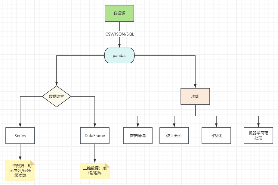
一、pandas 一、概要1. 简介pandas 是Python数据分析工具链中最核心的库，可用于数据读取、清洗、分析、统计、输出等，适用于处理结构化数据（如表格型数据）。2. 核心设计理念标签化数据结构：提供带标签的轴灵活处理缺失数据：内置NaN处理机制智能数据对齐：自动按标签对齐数据IO工具：支持CSV、Excel、SQL等多种数据源时间序列处理：原生支持日期时间处理和频率转换特性SeriesDataFrame维度一维二维索引单索引行索引 + 列名数据存储同质化数据类型各列的数据类型可以不同类比Excel 单列Excel Sheet创建方式pd.Series([1, 2, 3])pd.DataFrame({'col': [1, 2, 3]})